Register a Data Element

TL;DR

Register a column from a registered table as a Simple Data Element, or a value computed across multiple rows as an Aggregated Data Element. Once registered, it becomes a governed, versioned input that Features, Models, and Policies can consume.

What is it?

The Data Element Registry allows you to create a catalog of all available data points on the platform. Before a column in a DataTable can be used downstream, it must first be registered as a Data Element.

A Data Element acts as a governed layer between raw data columns and other registered objects:

flowchart LR
    Col["Raw column<br/>annual_inc"]:::raw --> DE["Data Element<br/>Annual Income"]:::de
    DE --> F["Features"]:::feature
    DE --> M["Models"]:::model
    DE --> P["Policies"]:::policy

    classDef raw     fill:#f9fafb,stroke:#9ca3af,color:#374151
    classDef de      fill:#f3f0ff,stroke:#9b7fe8,color:#3b1f8c,font-weight:600
    classDef feature fill:#f0faf4,stroke:#34a85a,color:#144d28
    classDef model   fill:#fffbea,stroke:#d4a017,color:#6b4c00
    classDef policy  fill:#fff4ec,stroke:#d4622a,color:#7a2e0e

Benefits of a registered Data Element

1. Enhanced data organization and documentation

Raw column names in DataTables are often hard to read (for example, annual_inc). By registering it as a Data Element, you can assign a meaningful alias, name, and description, building up a Data Dictionary that makes data easier to understand for new users.

2. Improved governance and control

• Apply permissible purpose tags to regulate Data Element usage (for example, marking gender or race as PII to restrict their use in marketing).
• Track versions of every change to the Data Element over time.
• Monitor downstream usage to see exactly where, and at which version, the Data Element is being consumed.

Two Types of Data Elements

A Data Element can be either Simple (a 1-to-1 mapping from a column) or Aggregated (a value computed across multiple rows).

	Simple	Aggregated
Maps from	A single column	Multiple rows across one or more tables
Use when	The column value is ready to use as-is	You need to compute something across records
Example	annual_income from app_table	Total bankruptcies in the last 10 years

You pick which kind to register by ticking or leaving the Is Aggregated checkbox in the Attributes section.

How to Register

The form has three sections: Attributes, Definition, and Properties. The Definition section changes depending on whether the Data Element is Simple (Is Aggregated unticked) or Aggregated (Is Aggregated ticked). Pick the matching tab below.

Simple Data ElementAggregated Data Element

Step 1: Open the Create Form

1. Open Data Vault → Data Element Registry from the home page.

2. Click + New Data Element at the top right.

   

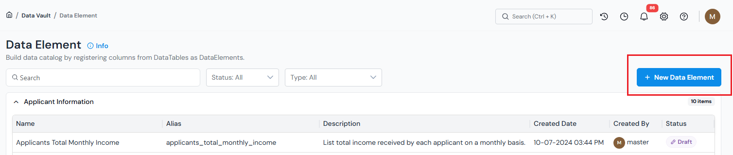
   Data Element Registry. Use + New Data Element to start a new entry.

3. Type a clear, descriptive name at the top of the form (for example, Account Vintage In Years) and click ✓.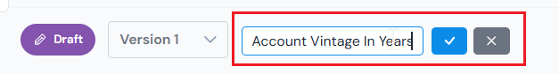

   

   Give the Data Element a descriptive name.

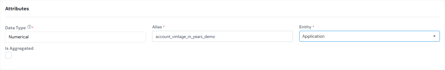
Step 2: Fill in Attributes

Leave Is Aggregated unticked.

Field	What to enter
Data TypeRequired	The type of value stored (for example, numerical, string, boolean, date).
AliasRequired	Short identifier used across the platform (for example, annual_income).
EntityRequired	Prospect, Application, Account, or Customer.
Is Aggregated	Leave unticked.

For a Simple Data Element, leave Is Aggregated unticked and fill in Data Type, Alias, and Entity.

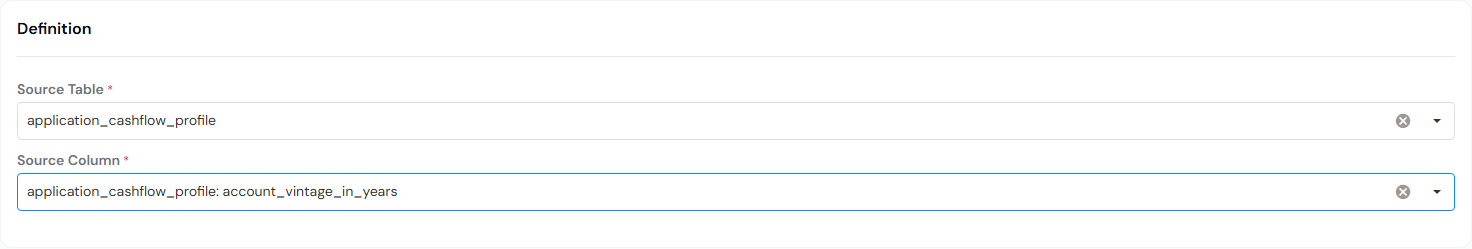
Step 3: Fill in Definition

Point at the column you want to expose.

Field	What to enter
Source TableRequired	The registered DataTable that contains the column.
Source ColumnRequired	The specific column to map.

Point the Data Element at the registered table and column it should expose.

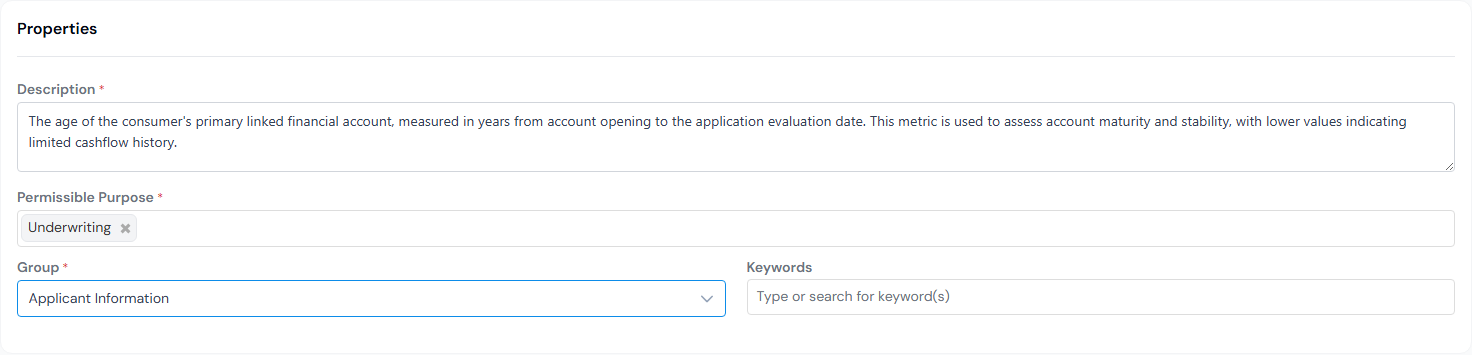
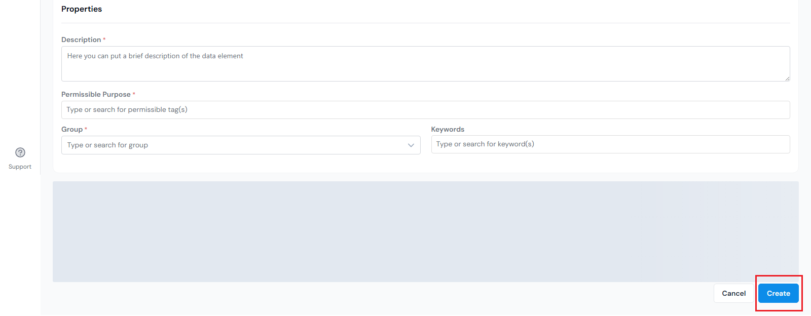
Step 4: Fill in Properties

Field	What to enter
DescriptionRequired	Plain-language explanation of what the Data Element represents. This is the entry that appears in your Data Dictionary.
Permissible PurposeRequired	Tags that control where the Data Element may be used (for example, PII, marketing-allowed).
GroupRequired	Logical grouping for the Data Element, used for display and organising similar use cases.
Keywords	Free-form tags that help search for the Data Element later.

Properties enrich the entry in the Data Dictionary and govern where the Data Element can be used.

Step 5: Click Create

Click Create at the bottom right of the form. The Data Element is saved as a draft and you land on its details page.

Submitting the form saves the Data Element as a draft and opens its details page.

Step 1: Open the Create Form

1. Open Data Vault → Data Element Registry from the home page.

2. Click + New Data Element at the top right.

   

   Data Element Registry. Use + New Data Element to start a new entry.

3. Type a clear, descriptive name at the top of the form (for example, Total Deposit Amount (Last 90D)) and click ✓.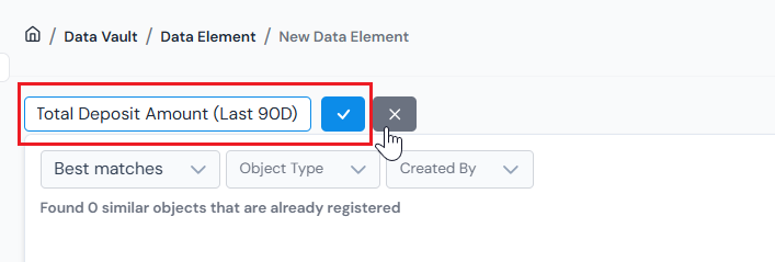

   

   Give the aggregated Data Element a descriptive name (for example, Total Deposit Amount Last 90D).

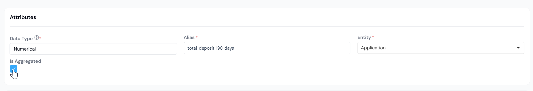
Step 2: Fill in Attributes

Tick Is Aggregated. The Definition section reveals an Input Type editor in place of the Source Column dropdown.

Field	What to enter
Data TypeRequired	The output type of your aggregation (for example, numerical for a count or a sum, boolean for a flag). There is no single source column for an aggregated Data Element.
AliasRequired	Short identifier (for example, bankruptcies_last_10y).
EntityRequired	The entity to group by (for example, Customer).
Is Aggregated	Ticked.

Tick Is Aggregated to switch the Definition section into aggregation mode.

Picking the right Data Type

The Data Type must match what your code returns:

• Counting rows or summing amounts → Numerical
• Returning a list of values → Array Numerical (or Array String, etc.)
• Returning a flag or category label → String or Boolean

The platform validates the return value against this type when you save.

Step 3: Fill in Definition

Ticking Is Aggregated in Step 2 is what reveals the Input Type editor in this section, replacing the Source Column dropdown.

Field	What to enter
Source TablesRequired	One or more tables linked to the entity. Each chosen table becomes a variable in the editor: a table aliased account is referenced as account in code.
Source ColumnsRequired	The specific columns from those tables that your aggregation reads. Each one is exposed inside the corresponding table variable.
Input	Any reusable global function registered on the platform that the aggregation should call.
Input Type	Pick the language used for the aggregation (Python, Pandas, or Spark), then write the logic in the editor below.

Source Tables and Source Columns feed the aggregation; the Input Type selector picks the language.

How the platform groups data

When you set Entity to Customer, and pick account (an Account-level table) as the source, Account rolls up to Customer. The platform groups Account rows by Customer before handing them to your code. Python and Pandas receive the data already filtered to one customer's rows, so you write logic for a single entity. Spark receives the full source table and you must do the groupBy('customer_id') yourself, returning a DataFrame keyed by the entity.

The editor supports three input languages. Pick the one that fits how you want to work with the data:

PythonPandasSpark

Python Input Type exposes each table as a dictionary of lists, already filtered to the current entity.

When you select Python as the Input Type, each source table is exposed as a dictionary of lists, sliced to the rows belonging to the current entity. Each column lookup returns a Python list. You can import standard libraries (numpy, math, datetime, etc.) inside the editor.

Example 1: Total number of accounts for customer

Inputs:

• Source Tables: account
• Source Columns: account_id

Only account_id is selected, so that is the only key available inside account. The platform hands your code a dictionary that looks like this:

account = {
    'account_id': [101, 102, 103],
}

Then your aggregation runs on top of it:

# `account` is a data dictionary
return len(set(account['account_id']))

Example 2: Default in the next 12 months of application

Inputs:

• Source Tables: account, account_performance
• Source Columns: account.account_application_date, account_performance.record_date, account_performance.charge_off_amount

Each table is its own dictionary, with one key per selected column. The platform hands your code the data sliced to one application's rows:

import datetime

account = {
    'account_application_date': [datetime.date(2024, 1, 15)],
}
account_performance = {
    'record_date':        [datetime.date(2024, 4, 1), datetime.date(2024, 8, 15), datetime.date(2025, 3, 1)],
    'charge_off_amount':  [None,                       500,                        None],
}

Then your aggregation runs on top of it:

import datetime

# sum charge_off_amount for records within 1 year of `account_application_date`
application_date = account['account_application_date'][0]
total_charge_off_amount = 0
for date, co_amt in zip(
    account_performance['record_date'],
    account_performance['charge_off_amount'],
):
    if (
        date >= application_date
        and date - application_date < datetime.timedelta(days=365)
        and co_amt
    ):
        total_charge_off_amount += co_amt

# default flag if total_charge_off_amount > 0
if not total_charge_off_amount:
    return 0
elif total_charge_off_amount > 0:
    return 1
else:
    return 0

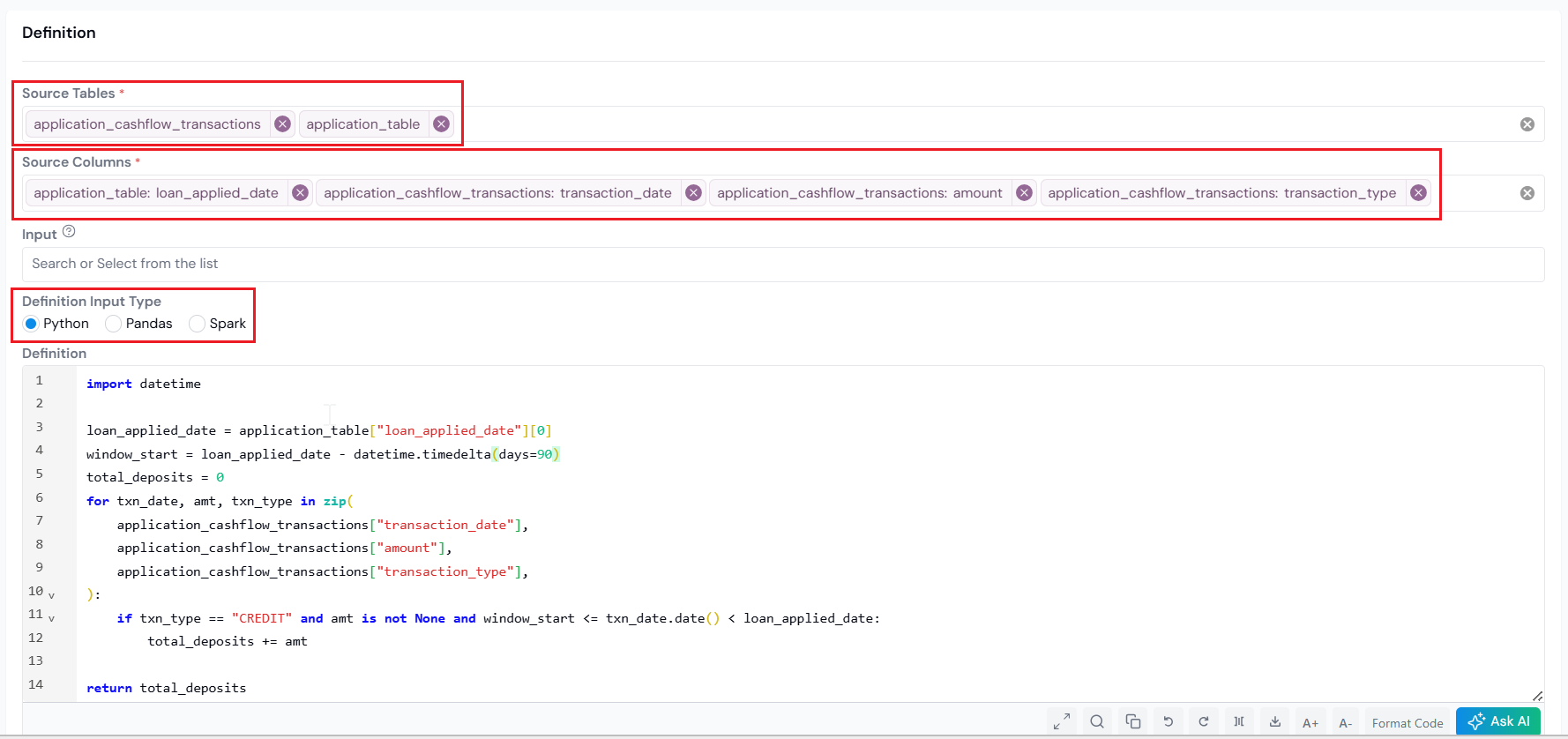
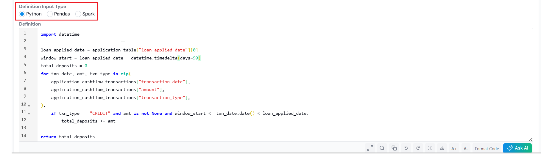
Example 3: Total deposit amount in the 90 days before application

Inputs:

• Source Tables: application_table, application_cashflow_transactions
• Source Columns: application_table.loan_applied_date, application_cashflow_transactions.transaction_date, .amount, .transaction_type

The Entity here is Application, so both dictionaries are sliced to one application's rows. The platform hands your code the data like this:

import datetime

application_table = {
    'loan_applied_date': [datetime.date(2025, 4, 1)],
}
application_cashflow_transactions = {
    'transaction_date':  [datetime.datetime(2025, 1, 15), datetime.datetime(2025, 2, 20), datetime.datetime(2025, 3, 10)],
    'amount':            [200,                              500,                            300],
    'transaction_type':  ['CREDIT',                         'DEBIT',                        'CREDIT'],
}

Then your aggregation runs on top of it:

import datetime

loan_applied_date = application_table["loan_applied_date"][0]
window_start = loan_applied_date - datetime.timedelta(days=90)
total_deposits = 0
for txn_date, amt, txn_type in zip(
    application_cashflow_transactions["transaction_date"],
    application_cashflow_transactions["amount"],
    application_cashflow_transactions["transaction_type"],
):
    if (
        txn_type == "CREDIT"
        and amt is not None
        and window_start <= txn_date.date() < loan_applied_date
    ):
        total_deposits += amt

return total_deposits

Pandas Input Type exposes each table as a DataFrame, already filtered to the current entity.

When you select Pandas as the Input Type, each source table is exposed as a pandas DataFrame, sliced to the rows belonging to the current entity. Column lookups return pandas Series.

Example 1: Total number of accounts for customer

Inputs:

• Source Tables: account
• Source Columns: account_id

Only account_id is selected, so account is a single-column DataFrame. The platform hands your code a DataFrame that looks like this:

# `account`:
#    account_id
# 0         101
# 1         102
# 2         103

Then your aggregation runs on top of it:

# `account` is a pandas DataFrame
return account['account_id'].nunique()

Example 2: Default in the next 12 months of application

Inputs:

• Source Tables: account, account_performance
• Source Columns: account.account_application_date, account_performance.record_date, account_performance.charge_off_amount

Each table becomes its own DataFrame, holding only the selected columns and only the rows for the current customer. The platform hands your code DataFrames that look like this:

# `account`:
#    account_application_date
# 0               2024-01-15

# `account_performance`:
#    record_date  charge_off_amount
# 0   2024-04-01                NaN
# 1   2024-08-15              500.0
# 2   2025-03-01                NaN

Then your aggregation runs on top of it:

import datetime

# get the account records with `record_date` within 1 year of `account_application_date`
application_date = account['account_application_date'].iat[0]
account_perf_within_1_year = account_performance[
    (application_date < account_performance['record_date']) &
    (account_performance['record_date'] - application_date < datetime.timedelta(days=365))
]

# drop the records that don't have a charge-off amount
account_perf_with_co_amt = account_perf_within_1_year.dropna(subset=['charge_off_amount'])

if account_perf_with_co_amt.empty:
    return 0
if account_perf_with_co_amt['charge_off_amount'].sum() > 0:
    return 1
else:
    return 0

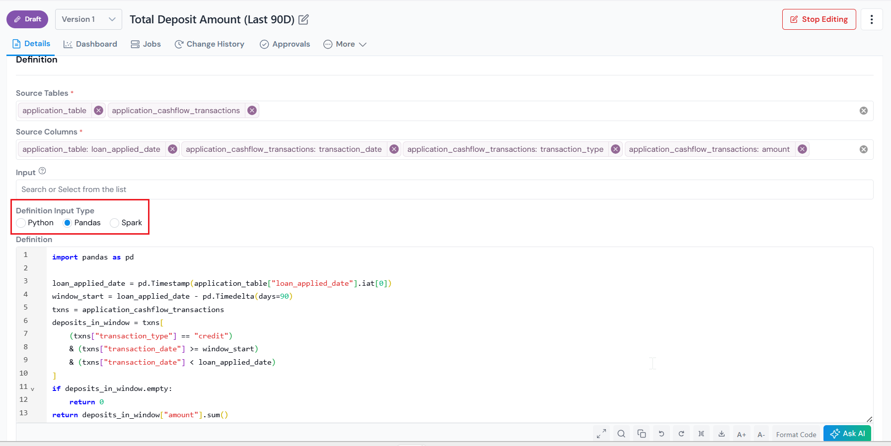
Example 3: Total deposit amount in the 90 days before application

Inputs:

• Source Tables: application_table, application_cashflow_transactions
• Source Columns: application_table.loan_applied_date, application_cashflow_transactions.transaction_date, .amount, .transaction_type

Entity is Application, so both DataFrames are sliced to one application's rows. The platform hands your code DataFrames that look like this:

# `application_table`:
#    loan_applied_date
# 0         2025-04-01

# `application_cashflow_transactions`:
#     transaction_date  amount  transaction_type
# 0         2025-01-15     200            credit
# 1         2025-02-20     500             debit
# 2         2025-03-10     300            credit

Then your aggregation runs on top of it:

import pandas as pd

loan_applied_date = pd.Timestamp(application_table['loan_applied_date'].iat[0])
window_start = loan_applied_date - pd.Timedelta(days=90)

txns = application_cashflow_transactions
deposits_in_window = txns[
    (txns['transaction_type'] == 'credit')
    & (txns['transaction_date'] >= window_start)
    & (txns['transaction_date'] < loan_applied_date)
]

if deposits_in_window.empty:
    return 0
return deposits_in_window['amount'].sum()

Spark Input Type exposes each table as an ungrouped DataFrame across all entities. The Output Dataframe Key field sits below the editor.

When you select Spark as the Input Type, each source table is exposed as a Spark DataFrame containing the full, ungrouped table across every entity. You do the groupBy yourself in code, and the return value must be a 2-column DataFrame: the entity key (for example, customer_id) and the aggregated value.

Example 1: Total number of accounts for customer

Inputs:

• Source Tables: customer_to_account
• Source Columns: customer_id, account_id

Spark hands you the full table across every customer:

# `customer_to_account`:
+-----------+----------+
|customer_id|account_id|
+-----------+----------+
|         42|       101|
|         42|       102|
|         42|       103|
|         43|       201|
|         43|       202|
+-----------+----------+

Then your aggregation runs on top of it, doing the groupBy yourself:

import pyspark.sql.functions as F

# `customer_to_account` is a Spark DataFrame
return customer_to_account.groupBy('customer_id').agg(
    F.countDistinct('account_id')
)

Example 2: Default in the next 12 months of application

Inputs:

• Source Tables: account, account_performance
• Source Columns: account.account_id, account.application_date, account_performance.account_id, account_performance.record_date, account_performance.COAMT

Both tables arrive ungrouped, with the join key included so you can stitch them together. The platform hands your code DataFrames that look like this:

# `account`:
+----------+----------------+
|account_id|application_date|
+----------+----------------+
|       101|      2024-01-15|
|       201|      2024-02-10|
+----------+----------------+

# `account_performance`:
+----------+-----------+-----+
|account_id|record_date|COAMT|
+----------+-----------+-----+
|       101| 2024-04-01| null|
|       101| 2024-08-15|  500|
|       201| 2024-05-20| null|
+----------+-----------+-----+

Then your aggregation runs on top of it:

import pyspark.sql.functions as F
from pyspark.sql.functions import udf
from pyspark.sql.types import IntegerType

acc_perf = account_performance.select(
    'account_id', 'record_date', 'COAMT'
).join(
    account.select('account_id', 'application_date'),
    on='account_id', how='left',
)

CO1yr_df = acc_perf.filter(
    acc_perf.record_date < F.date_add(acc_perf['application_date'], 365)
)
COAMT_df = (
    CO1yr_df.groupBy('account_id')
    .agg(F.sum('COAMT'))
    .toDF('account_id', 'COAMT')
)

def charge_off(x):
    return 1 if x > 0 else 0

charge_off_flag_udf = udf(lambda s: charge_off(s), IntegerType())

COAMT_df = COAMT_df.withColumn(
    'charge_off_flag', charge_off_flag_udf('COAMT')
)

return COAMT_df.select('account_id', 'charge_off_flag')

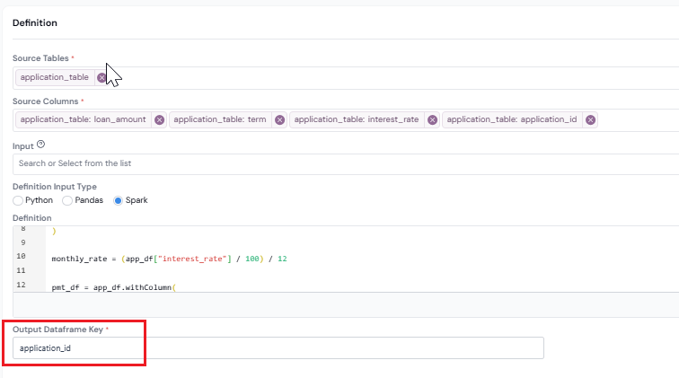
Example 3: Total deposit amount in the 90 days before application

Inputs:

• Source Tables: application_table, application_cashflow_transactions
• Source Columns: application_table.application_id, application_table.loan_applied_date, application_cashflow_transactions.application_id, .transaction_date, .amount, .transaction_type

Full unfiltered tables across all applications. The platform hands your code DataFrames that look like this:

# `application_table`:
+--------------+-----------------+
|application_id|loan_applied_date|
+--------------+-----------------+
|          A001|       2025-04-01|
|          A002|       2025-04-05|
+--------------+-----------------+

# `application_cashflow_transactions`:
+--------------+----------------+------+----------------+
|application_id|transaction_date|amount|transaction_type|
+--------------+----------------+------+----------------+
|          A001|      2025-01-15|   200|          CREDIT|
|          A001|      2025-02-20|   500|           DEBIT|
|          A001|      2025-03-10|   300|          CREDIT|
|          A002|      2025-02-25|   400|          CREDIT|
+--------------+----------------+------+----------------+

Then your aggregation runs on top of it. Join on application_id, filter, then aggregate back to one row per application:

import pyspark.sql.functions as F

txns = application_cashflow_transactions.join(
    application_table.select('application_id', 'loan_applied_date'),
    on='application_id', how='left',
)

deposits_in_window = txns.filter(
    (F.col('transaction_type') == 'CREDIT')
    & (F.to_date('transaction_date') >= F.date_sub(F.col('loan_applied_date'), 90))
    & (F.to_date('transaction_date') < F.col('loan_applied_date'))
)

return deposits_in_window.groupBy('application_id').agg(
    F.sum('amount').alias('total_deposits_last_90d')
)

Spark constraints

• SELECT only. Use SELECT queries on the input tables. CREATE, INSERT, DROP, and similar mutations are not allowed.
• No external data reads. Do not read from outside sources with spark.read.csv, spark.read.parquet, or similar. Use only the tables provided as inputs.
• Self-contained logic. Each Data Element's code must run on its own. Do not depend on intermediate state from another Data Element.
• No cross-Data-Element UDFs or temp views. UDFs and temp views registered in one Data Element must not be used in another.

Set the Output Dataframe Key

Spark adds an extra Output Dataframe Key field below the editor. Enter the name of the entity key column in your returned DataFrame (for example, customer_id, account_id, or application_id). The platform uses this to join the aggregation result back to the parent entity.

Specify the entity key column in Output Dataframe Key so the platform can join the aggregation back to the parent entity.

Enter the exact name of the entity key column in the DataFrame your code returns.

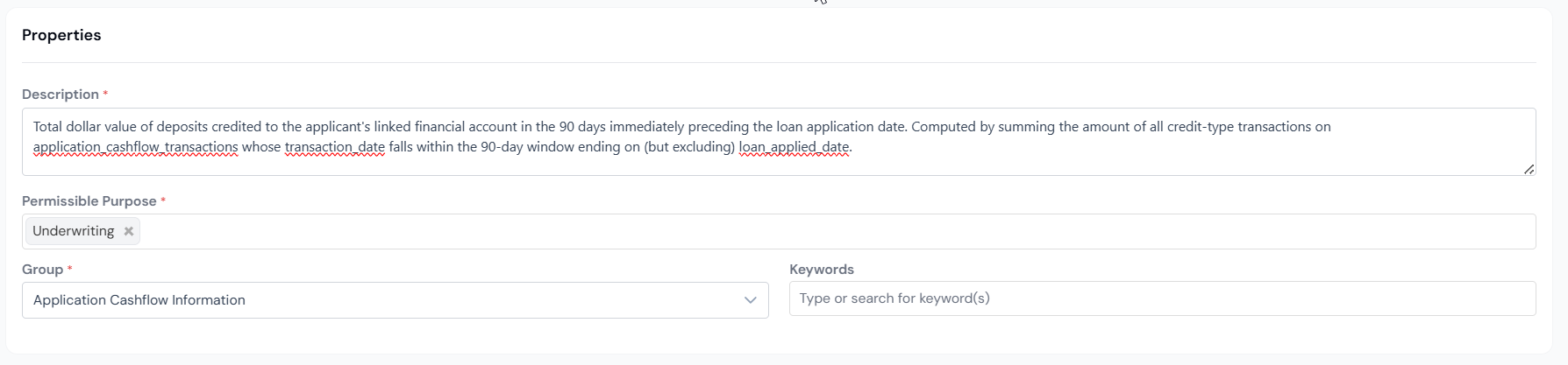
Step 4: Fill in Properties

Field	What to enter
DescriptionRequired	Plain-language explanation of what the Data Element represents.
Permissible PurposeRequired	Tags that control where the Data Element may be used.
GroupRequired	Logical grouping for the Data Element, used for display and organising similar use cases.
Keywords	Free-form tags for search.

Properties enrich the entry in the Data Dictionary and govern where the Data Element can be used.

Step 5: Click Create

The Data Element is saved as a draft and you land on its details page.

How can it be used?

Once registered, you can:

• Run a simulation on the Data Element to generate basic summary statistics, such as min, max, mean, and percentage of missing values.
• Use the Data Element downstream in Features, Models, Policies, and other registered objects.
• Track its lineage to see every place the Data Element flows into.

What's Next

• Build a Feature on top of this Data Element.
• Send the Data Element for approval so it can be used outside your draft workspace.